3. Human perception of colours
Human vision system is sensitive a certain range of frequencies. Radiations out of that range are not visible. In daylight, we perceive different colours depending on received spectral distribution: three types of cells in our retina are exited with different level.
Tristimulus is a mathematical basis for representing a mix of three primaries. It would seem a natural way of characterising reflectance and illumination: we use colour primaries in photography and cinema. We are familiar with red, green and blue, or cyan, magenta and yellow primaries.
But a colour or tristimulus value does not defines a unique spectrum: we can perceive multiple spectra as the same colour. This is called metamerism. This is not a concern for photography: we are interested by the image resulting of the physical transport of light. It reproduces what our eyes would see. It is however a concern for computer graphics where we simulate light transport.
In this chapter, we discuss the importance of spectral consideration for reflectance and illuminant in computer graphics.
The first section introduces photometric units and how spectra are perceived as colours. We show example of metamerism.
In the second section we compare tristimulus rendering with spectral rendering. We discuss the reasons for tristimulus wide adoption in computer graphics and motivate the need for a spectral rendering pipeline transition.
We need to characterise the energy distribution when simulating light transport. Using tristimulus values can lead to serious discrepancies. Light is reflected depending on its spectral distribution not depending on a set of primaries. Tristimulus values, and colour in particular, are perceptual concepts and mathematical framework resulting of physics and biology. They do not characterise a physical wavelength distribution.
Human vision and Tristimulus
Photometry
The retinas at the back of the human eye are composed by two different types of photosensitive cells, rods and cones. Both are used for vision, depending on lighting conditions.
-
In bright environments, cone cells are active. This is called photopic vision. The human eye have three types of cones sensitive to different frequencies; S for small-wavelength-sensitive, M for middle-wavelength-sensitive, L for long-wavelength-sensitive. This allows colour vision.
-
In lower brightness conditions, rod cells are active. This is called scotopic vision. Rod cells are more sensitive than cone cells. Rod cells share the same sensitivity range hence we are unable to distinguish colours in a darker environment.
Cone and rod cells having different sensitivity bandwidth, vision varies depending on lighting condition. This is described by the luminosity function (Figure 1) and varies depending on the lighting condition.

We use photometric units quantities to describe how much of the light is perceived. It is an equivalent of radiometric units, characterising radiation, for perception (see Table bellow).
| Name | Symbol | Units | Radiometric equivalent |
|---|---|---|---|
| luminous flux | \(\Phi_v\) | lumen \([\mathrm{lm}]\) | radiant flux |
| illuminance | \(E_v\) | lux \([\mathrm{lx}]\) i.e. \([\mathrm{lm.m^{-2}}]\) | irradiance |
| luminous intensity | \(I_v\) | candela \([\mathrm{lm}]\) i.e. \([\mathrm{lm.sr^{-1}}]\) | radiant intensity |
| luninance | \(L_v\) | nits \([\mathrm{cd.m^{-2}}]\) i.e. \([\mathrm{lm.m^{-2}.sr^{-1}}]\) | radiance |
To convert from radiance \(L_e\) to the luminance \(L_v\), we use the following equation for photopic vision (daytime):
\[\begin{equation} L_v = K_m \int_\Lambda L_e(\lambda) V_M(\lambda) \:\mathrm{d} \lambda \qquad [\mathrm{lm.m^{-2}.sr^{-1}}] \label{eqn:photopic} \end{equation}\]With: \(K_m = 683 \mathrm{lm.W^{-1}}\), the maximum luminous efficacy for photopic vision.
For scotopic vision (dim-light):
\(\begin{equation} L_v = K'_m \int_\Lambda L_e(\lambda) V(\lambda) \:\mathrm{d} \lambda \qquad [\mathrm{lm.m^{-2}.sr^{-1}}] \label{eqn:scotopic} \end{equation}\) With: \(K_m = 1700 \mathrm{lm.W^{-1}}\), the maximum luminous efficacy for scotopic vision.
We have to specify the luminous efficiency function corresponding to the environment when we use a photometric unit.
Determining colour primaries
The theory of colour vision based on primaries started with Newton [Newton 1704]. He stated that seven primaries (red, orange, yellow, green, blue, indigo and violet) can be mixed to reproduce any visible colours. He based his theory on the observation of the sun light dispersed by a prism. Later, mathematical and experimental foundation was refined by Young [Young 1802b], [1802a], Grassmann [Grassmann 1853] Helmholtz [Helmholtz 1852] [1855] and Maxwell [Maxwell 1857], [1860] with the theory of three primaries.
To determine the visual sensitivity to light, the Commission Internationnale de l’Éclairage (CIE), conducted a series of experiments from 1920 to lead to the CIE 1931 XYZ colour space. The CIE 1931 \(2^{\circ}\) colour matching functions (CMFs) are based on the CIE 1924 \(V(\lambda)\) photopic luminosity function. This photopic luminosity function underestimate the importance of eye sensitivity below 460 nm. Stiles and Burch re-conduct the experiment to refine the CMFs among 10 observers for \(2^{\circ}\) matching field [Stiles and Burch 1955] and for \(10^{\circ}\) matching field [Stiles and Burch 1959].

An observer was facing a screen with two patches of light and a series of three knobs. One patch, the reference, is made of a monochromatic light and the observer have to manipulate the knobs controlling the amount of three primaries of almost monochromatic lights to match the colour of the second patch with the reference (\(r = 648.6\:\mathrm{nm}\), \(g = 526.4\:\mathrm{nm}\), \(b = 445.3\:\mathrm{nm}\) in the CIE 1931, \(r = 645.2\:\mathrm{nm}\), \(g = 526.3\:\mathrm{nm}\), \(b = 444.4\:\mathrm{nm}\) in (Stiles and Burch 1955, 1959)). To match some colours, negative values have to be used for the knobs. A negative position on the knob is simulated by adding the corresponding opposite value to the reference patch. Figure 2 shows the resulting curves for the colour-matching function.

To overcome the problem of having negative RGB coordinates, the CIE proposed the CIE 1931 \(2^{\circ}\) XYZ colour space. Similar to Stiles and Burch RGB corrected visibility function for \(V(\lambda)\) below 460nm, Judd [Judd 1951] and later Vos [Vos 1978] proposed a correction for CIE 1931 \(2^{\circ}\) XYZ. More recently, the CIE released CIE 2006 XYZ colour matching functions based on cone fundamentals from Stockman and Sharpe [Stockman and Sharpe 2000] (see Figure 3).
Reflectance and colours
| D65 | FL4 | A | |
|---|---|---|---|
| SPD |  |
 |
 |
| Macbeth |  |
 |
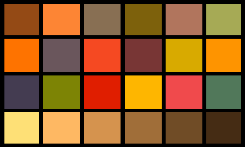 |
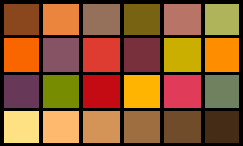
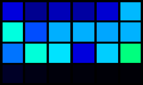
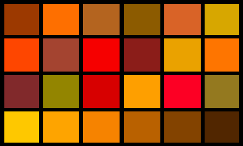
When characterising a reflectance by its colour, it is important to also specify under which illuminant it is observed. For example, Figure 4 shows a Macbeth colour checker lit by different illuminants. The illuminant used to lit the scene drastically influences the perceived colours of the patches. Under D65, some patches appear blue while they are looking violet under fluorescent illuminant FL4.
From spectra to tristimulus
To transform a spectra into a perceived colour, we use colour matching functions. Usually, we first transform spectra to XYZ coordinates. Then, we transform XYZ coordinates to a specific colour space depending on the targeted application.
In computer graphics, we typically display an image on a 8bit RGB monitor. We transform XYZ to RGB values, then gamma correct to sRGB.
Radiance
To get XYZ coordinates of a radiance spectrum, we multiply and integrate the spectral radiance with the colour matching functions:
\[\begin{aligned} \begin{cases} \displaystyle X = \int_\Lambda L_e(\lambda) \bar{x}(\lambda) \:\mathrm{d} \lambda\\ \displaystyle Y = \int_\Lambda L_e(\lambda) \bar{y}(\lambda) \:\mathrm{d} \lambda\\ \displaystyle Z = \int_\Lambda L_e(\lambda) \bar{z}(\lambda) \:\mathrm{d} \lambda \end{cases} \end{aligned}\]Notice from equation \eqref{eqn:photopic}, the luminance can be retrieved from the \(Y\) component in photopic conditions by multiplying it with the corresponding \(K_m\).
Reflectance
We mentioned in section 1.3 the perceived colour of reflectance depends on the illumination under which it is observed. Then, we specify XYZ coordinates of a reflectance relative to an illuminant:
\[\begin{aligned} &\begin{cases} \displaystyle X = \frac{1}{N}\int_\Lambda s(\lambda) L_e(\lambda) \bar{x}(\lambda) \:\mathrm{d} \lambda \\ \displaystyle Y = \frac{1}{N}\int_\Lambda s(\lambda) L_e(\lambda) \bar{y}(\lambda) \:\mathrm{d} \lambda \\ \displaystyle Z = \frac{1}{N}\int_\Lambda s(\lambda) L_e(\lambda) \bar{z}(\lambda) \:\mathrm{d} \lambda \end{cases} \end{aligned}\]With \(N = \int_\Lambda L_e(\lambda) \bar{y}(\lambda) \:\mathrm{d} \lambda\).
Where:
- \(L_e(\lambda)\) is the spectral radiance of the illuminant.
- \(s(\lambda)\) is the spectral reflectance.
Metamerism
A spectrum defines a colour, but a colour does not define an unique spectra: multiple spectra can lead to the observation of the same colour due to the way humans perceive colours. In mathematical terms, there is a surjection between spectra and colours.

| HP1 | D65 | |||
| SPD |  |
|
||
| Original | Metamer | Original | Metamer | |
| Colour patches |  |
 |
 |
 |
While some patches have a clear colours difference in Figure 4 under D65 (green and yellow), it is much harder to see the difference between the same patches under FL4 or A illuminants. The extreme cases is when two different reflectance spectra appears the same under a given illuminant. They are then called metamers under this illuminant. When changing illuminant, the difference between the reflectance may appear.


In practice, metamers can easily appear when two surfaces are lit with purely monochromatic light. If the surface is not fluorescent, it only reflects the incoming wavelength (see Figure 6). This is typically the case with street lighting using low pressure sodium-vapour lamps which are nearly monochromatic.
Figure 5 shows a example of two metamers for a given illuminant. One reflectance is taken from one of the Macbeth colour checker. The second reflectance is synthetically generated to produce the same perceived colour under HP1 illuminant.
Spectral and tristimulus pipelines
A colour does not properly define an illuminant or a reflectance due to metamerism. Still, many rendering pipelines rely on tristimulus values, whether renderers, or softwares used by artists to edit textures, for multiple reasons:
-
Efficiency
In the early days, with limited computational resources, the exclusive usage of tristimulus values enabled producing colour images with reasonable compromise on accuracy. A consequence of this long-term usage is the knowledge acquired on weaknesses and drawbacks of the tristimulus pipeline. -
Transition
From a software point of view, moving from a tristimulus to a spectral workflow would imply an important codebase adaptation. Years of development resulted in software working correctly in tristimulus with known weaknesses. Transitioning to spectral would potentially break many features. -
Intuitiveness
For artists, it is no easy task to switch from colours to spectra paradigm, the latter being far less intuitive to work with.
Tristimulus renderers are approximative. In some circumstances, they produce images very different from what a real scene would look like. This is especially problematic for prototyping applications. An architect or a car manufacturer could have misleading information about the appearance of paints depending on lighting conditions.
In the following sections we review some of the approximations caused by tristimulus rendering.
The core approximation of a tristimulus renderer
In a spectral renderer, we treat each wavelength independently. We transform to tristimulus values only at the end of the evaluation. Each reflectance and illuminant have then to be specified as a spectrum.
In a tristimulus renderer, we treat each reflectance and illuminant as tristimulus values and multiply them. The integration transforming the spectra to tristimulus values is applied prior to the evaluation. In practice, the values are directly provided in XYZ or RGB and multiplied with each other.
Equation \eqref{eqn:approx_tristimulus} shows the core approximation made by a tristimulus renderer1. In this equation, we apply a normalisation factor to the illuminant. This results in a correct result only in the case of single bounce if the illuminant we use to lit the scene match the one we use for reflectance tristimulus values. In practice, the need for this correction factor is arguable:
-
If the illuminant is seen directly, this leads to incorrect colour result.
-
While getting accurate results in single bounce and same illuminant scenario, when changing illuminant, it can cause more discrepancies.
-
In a multiple bounce scenario, each element reflecting in the scene would act as a secondary light source. The re-normalisation factor is unpredictable and can increase the error.
Where:
- \(r(\lambda)\) is the spectral reflectance.
- \(L_e(\lambda)\) is the spectral power distribution of the illuminant for rendering.
- \(L^m_e(\lambda)\) is the spectral power distribution of the illuminant for measuring reflectance.
- \(\bar{c}(\lambda)\) is one of the colour matching functions $(\bar{x}, \bar{y}, \bar{z})$.
Comparing spectral and tristimulus rendering
We evaluate the approximation made by a tristimulus rendering pipeline influences the final appearance. We compare both methods:
-
In a single bounce context with variation of reflectance and illuminant. We use the Macbeth colour checker as the base collection of reflectance. Each patch is specified as a reflectance spectra. We show:
-
Colour discrepancies when using a different illuminant than the one used for measurement,
-
Limitations of tristimulus rendering threw reflectance and illuminant metamers.
-
-
In a global illumination context we show:
-
Energy conservation problems rising with tristimulus rendering with generated spectra,
-
Error accumulation after multiple bounces in a Cornell box,
-
Discrepancies depending on the colour matching function used for representing illuminant and reflectance.
-
Single bounce
Reflectance rendering under different illuminants
The illuminant influences the perceived colour of a reflectance. Figure 7 shows the impact of the pre-integration made in a tristimulus renderer on the colour accuracy using three different illuminants:
-
D65
is from the CIE series of daylight illuminants. This illuminant represent the average daylight illumination in Western Europe. Its spectral power distribution is well distributed and provides good ability for distinguishing colours. -
FL4
is from the CIE series of fluorescent illuminants. Also called F4, this illuminant corresponds to a fluorescent lighting. The CIE used FL4 for colour rendering index calibration. It has two peaks around 410 nm and 435 nm and a larger emission band from 520 nm to 650 nm. -
HP1
illuminant corresponds to a high-pressure vapour lamp. It has a narrow emission band roughly from 550 nm to 620 nm. It is difficult to differentiate colours under this illuminant.
For tristimulus rendering, we convert each patch of the colour checker to XYZ values as they would be measured under a given illuminant (here CIE D65). We convert the illuminant to XYZ values and correct it to match the measurement illuminant. We multiply the two XYZ sets together.
| Spectral rendering | Tristimulus rendering | \(\Delta E^*_{2000}\) | |
|---|---|---|---|
| D65 |  |
 |
 |
| a | b | \(\Delta E^*_{2000}(a, b)\) | |
| FL4 |  |
 |
 |
| a’ | b’ | \(\Delta E^*_{2000}(a', b')\) | |
| HP1 |  |
 |
 |
| a’’ | b’’ | \(\Delta E^*_{2000}(a'', b'')\) |
-
With D65, the illuminant matches the one used for measuring the reflectance, the tristimulus rendering is exact. This is expected since the integration is made during the measurement and then a simple scaling is applied depending on the relative power of the illuminant used for rendering.
-
With FL4, the error increase for the coloured patches. When reflectance spectrum have its most reflectivity in values within the re-radiation band of the FL4 illuminant (\(520\sim 630\:\mathrm{nm}\)), it can be well represented with a tristimulus renderer. The fluorescent lamp also have an emission peak around \(400\:\mathrm{nm}\) and around \(440\:\mathrm{nm}\). Those two peaks are going to misrepresented: mostly X and Z values are affected. Those two functions have a much larger bandwidth than the emission peaks. This explains the poor rendering accuracy of the blue part of the spectrum.
-
This high frequency phenomena is even more pronounced with HP1 illuminant: the emission band is narrow and cannot be well represented by multiplications with XYZ values.
-
The grey reflectance, on the bottom line, have good rendering accuracy in a tristimulus renderer. Their reflectance spectrum is almost constant. This limited dependence to wavelength explains the good rendering results regardless the illuminant used.
In conclusion, the error caused by a tristimulus renderer is limited when we have low frequency illuminant or reflectance spectra.
Reflectance metamers
A tristimulus renderer will not handle reflectance metamers. When observed under another illuminant, the reflectance will appear identical while they should differ according to their reflectance spectra: the same XYZ values are used in both cases even if reflectance spectra differs.
| Original | Metamers | \(\Delta E^*_{2000}\) | |
| Spectral |  |
 |
 |
| a | b | \(\Delta E^*_{2000}(a, b)\) | |
| Tristimulus | 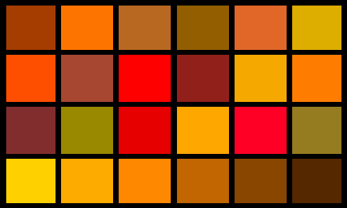 |
 |
 |
| a' | b' | \(\Delta E^*_{2000}(a', b')\) |
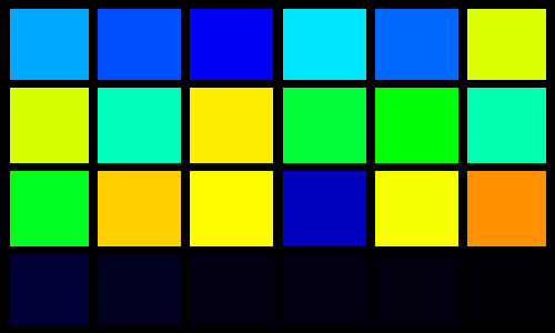
Figure 8 shows an example of two colour checkers. One is the original Macbeth colour checker. For the other, we replaced each of its patches by a metamer reflectance under an illuminant with a flat SPD. Only a spectral renderer accurately shows the difference between the two colour checkers depending on the illuminant.
Illuminant metamers
Similarly to metamer reflectance, we can generate metamer illuminant. If the illuminant is reflected by a perfectly grey surface (constant reflectance regardless the wavelength), the surface will appear the same to our eyes with both illuminants even though their emission spectra differ. Other reflectance are going to look different.

| D65 | D65 metamer | \(\Delta E^*_{2000}\) | |
| Spectral |  |
 |
 |
| a | b | \(\Delta E^*_{2000}(a, b)\) | |
| Tristimulus |  |
 |
 |
| a' | b' | \(\Delta E^*_{2000}(a', b')\) |
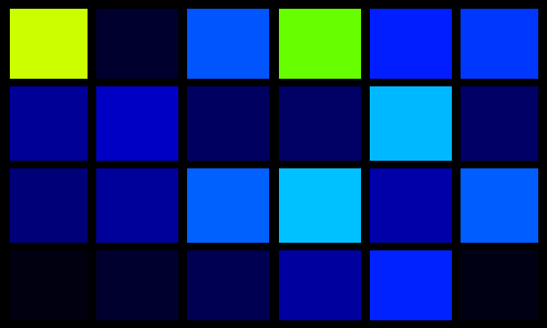
In Figure 9 we show a such scenario. We generate a metamer illuminant for D65. We then compare the Macbeth colour checker lit by the original D65 illuminant and its metamer.
-
With a spectral rendering, the patches have a different colour from one illuminant to the other. This is expected: the illuminants have different spectral power distributions.
-
With a tristimulus rendering, there is no difference when changing illuminant. The two metamer illuminants are transformed to the same XYZ values prior to the rendering.
Only a spectral renderer with spectral reflectance can handle metamer illuminants.
Global illumination
Global illumination increases the discrepancies exposed before. At each new reflection bounce event, a tristimulus renderer accumulates error.
Even if we specify all reflectance using the illuminant in the scene, each light bounce step is equivalent to a new illuminant radiating the next reflectance. This yields to incorrect results and breaks energy conservation, starting from the second light bounce.
Energy conservation
To illustrate the potential loss and creation of energy caused by a tristimulus renderer, we generate two synthetic cases:
-
In the first (see Figure 10.a), we simulate scattering from D65 illuminant to a patch and a second bounce from this first patch to another one having the same reflectance. The reflectance is perfectly reflecting the light between 440 nm and 550 nm. Otherwise, the light is absorbed. We observe a loss of energy in the case of a tristimulus renderer: the XYZ components of the reflectance cannot reflect the nature of the spectra.
-
In the second (see Figure 10.b), we use the first spectrum as the one used before. For the second bounce, we use a complementary spectrum: its reflectance is null at the value where the other spectrum reflects and perfectly reflective where the other absorbs light. We observe creation of energy in the case of a tristimulus renderer: not null XYZ values are multiplied together.
We do not attenuate the light depending on its angle nor considering the distance: we are only interested in showing the absence of energy conservation caused by the multiplication of XYZ values instead of spectra.
| Reflectance A | Reflectance B |
 |
|
 |
|
| Tristimulus renderer | |
 |
 |
| Spectral renderer | |
|
 |
| Reflectance A | Reflectance B |
|
 |
 |
 |
| Tristimulus renderer | |
 |
 |
| Spectral renderer | |
|
 |
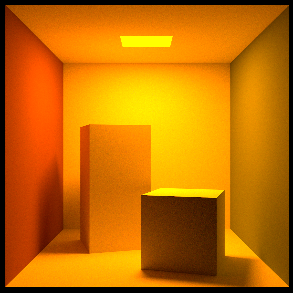
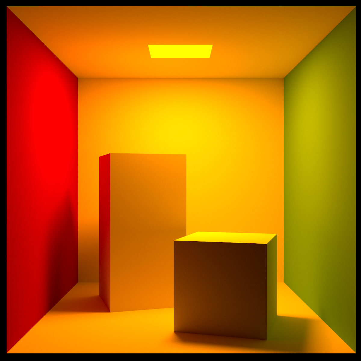
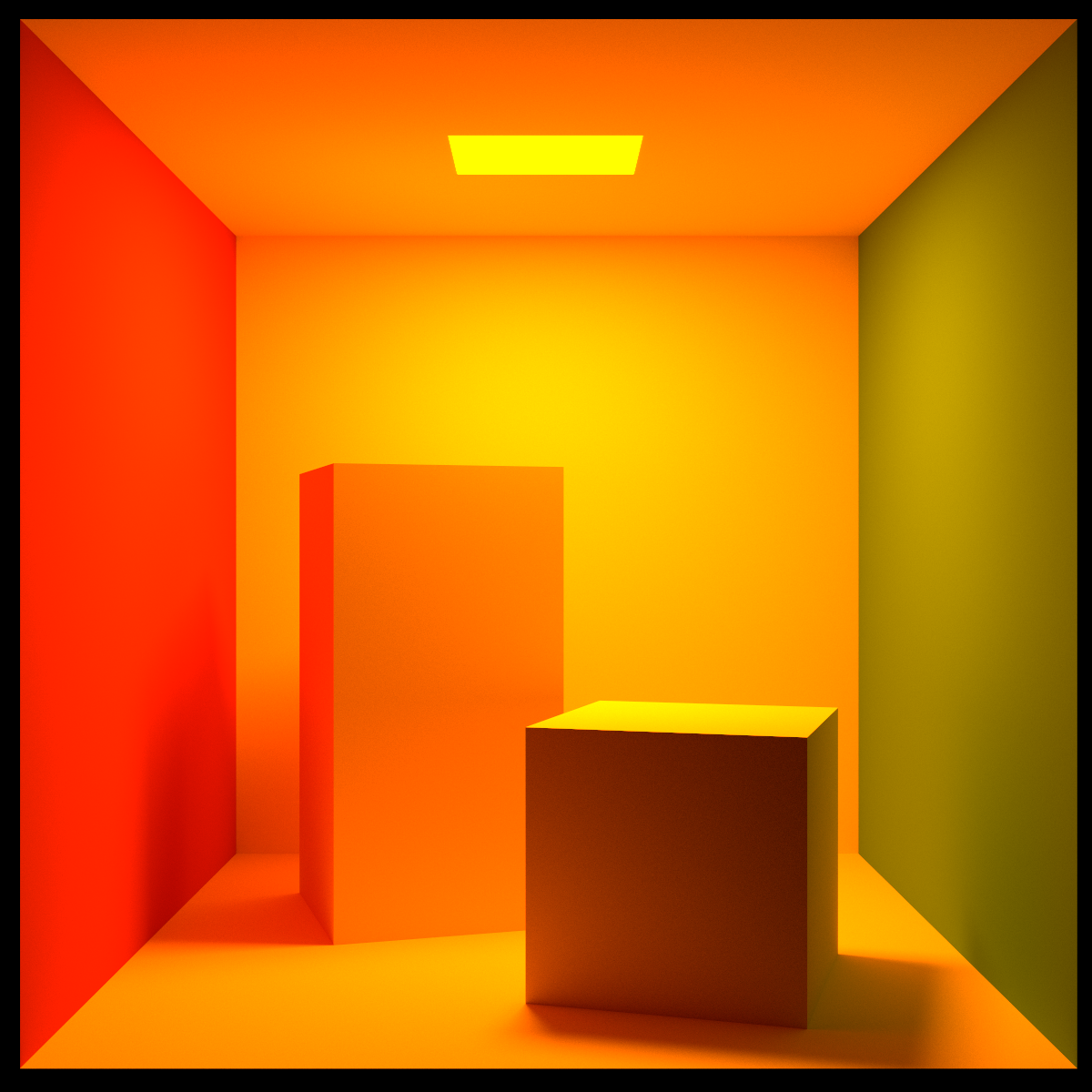
Cornell box example
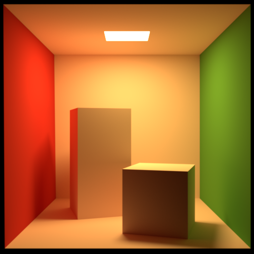
To show a practical example of discrepancies observable with a simple scene, we use the Cornell box rendered with Mitsuba [Jakob 2010]. The spectral variant is using 30 spectral samples while the tristimulus variant is converting all spectra to RGB prior to light transport.
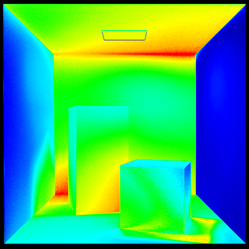
| Spectral | RGB | \(\Delta E^*_{2000}\) | |
| Spectral | 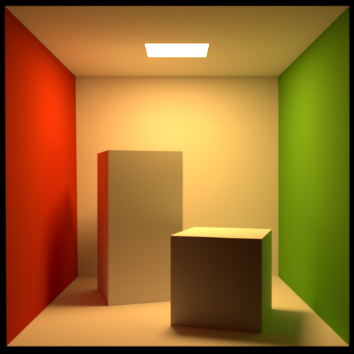 |
 |
 |
| a | b | \(\Delta E^*_{2000}(a, b)\) | |
| Tristimulus | 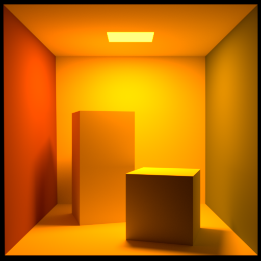 |
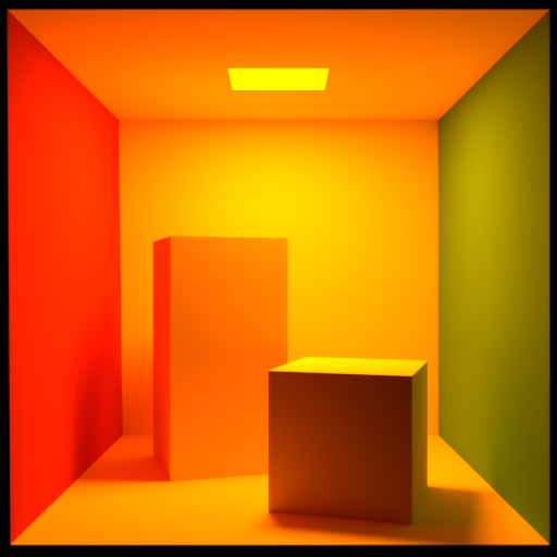 |
 |
| a' | b' | \(\Delta E^*_{2000}(a', b')\) |
The appearance drastically change if using tristimulus values instead of the full spectrum for rendering (see Figure 11).
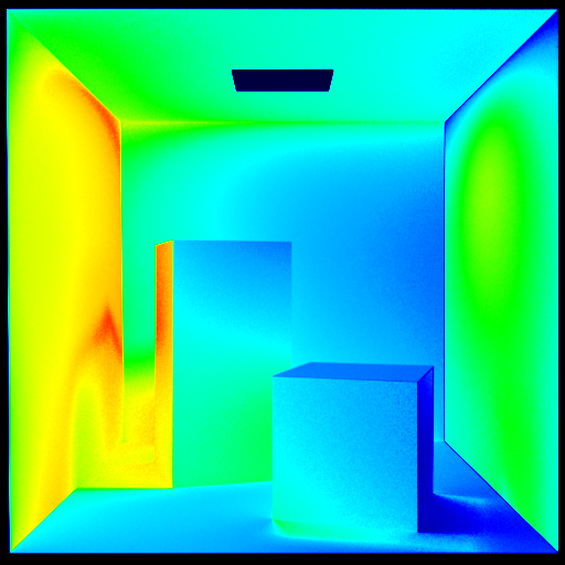
For the same input spectra, the colour matching functions used in a tristimulus renderer can also drastically change the appearance of the output image (see Figure 12)).
The error would significantly increase with multiple light sources having different spectra.
Discussion
Drawbacks of spectral rendering
The major drawback of a spectral renderer is the need to specify a spectrum for each illuminant and reflectance. Most tools provided to artists are designed with tristimulus in mind. Spectral uplifting overcomes this problem by creating plausible spectrum from tristimulus values. Jakob and Hanika [Jakob and Hanika 2019] recently proposed a method to convert tristimulus textures to plausible spectral reflectance.
Another drawback of a spectral renderer is its inefficiency. While a tristimulus renderer evaluates directly a colour, a spectral renderer adds a dimension to the evaluation. In a path tracer, it means, in addition to the ray direction sampling, the wavelength of the ray also have to be sampled. Usually, in a spectral path tracer, a ray carries a single wavelength. This results in colour noise in low sampled images. However, Hero Wavelength Spectral Sampling (HWSS) technique drastically limit this phenomena carrying multiple wavelengths as the same time with almost the same computational time taking advantage of Single Instruction Multiple Data (SIMD) hardware capabilities [Wilkie et al. 2014].
Advantages of spectral rendering
Spectral rendering is more accurate compared to its tristimulus counterpart, avoiding energy leaks. It also simulates effects impossible to handle correctly in a tristimulus renderer: light dispersion, fluorescence, and polarisation. Those effects are wavelength dependent and thus require consideration for spectra.
Metamerism is another major issue a tristimulus renderer cannot deal with. While two reflectance spectra can be different, their tristimulus counterparts can be the same under a given illuminant. Only a spectral renderer is able to show the difference between those two spectra when changing the illuminant.
Finally, a spectral renderer is agnostic to colour matching functions. The final image can be saved as a spectrum and later converted to a tristimulus display for instance an RGB monitor. The monitor colour response and the observer one can be applied directly to the spectral image to get correct colourimetry. On the other hand, a tristimulus image has to rely on chromatic adaptation.
Conclusion
We presented how light is perceived by the human vision system and experiments at the origin of the colour matching functions used for transforming spectra to tristimulus coordinates. We use XYZ coordinates to avoid negative values. Starting from these coordinates, we convert to different colour spaces depending on the application. In computer graphics, we mostly use RGB primaries.
For computer graphics applications, tristimulus representations have a major limitation: different spectra can be represented with the same tristimulus coordinates. This can result in important discrepancies using tristimulus rendering pipelines. Spectral rendering is immune to this problem.
However, moving a well-established tristimulus pipeline to spectral is challenging. It requires important code rewriting. We have to specify each reflectance and illuminant in their spectral form. Editing software used by artists are not yet suited for spectral application and using spectral paradigm instead of colour is less intuitive.
Finally, material acquisition is usually performed using tristimulus coordinates. Recently, efficient spectral acquisition techniques were proposed for non-spatially varying materials. For spatially varying material, is out of reach though at the time of writing this thesis. Storage and acquisition time issues, already problematic with tristimulus representations, would drastically increase.
Tristimulus rendering offers a decent approximation in most of the cases and provides efficient evaluation. For critical applications, it is important to be well aware of its limitations though. We cannot use it with line spectra (low pressure vapour lamps for instance) and it is incapable of handling metamers. Particular wavelength dependent effects such as fluorescence and polarisation are also out of reach for a tristimulus renderer.
Sources & references
Datasets
-
Colour matching functions: The Colour & Vision Research Laboratory
https://www.rit.edu/science/munsell-color-lab -
Illuminants: The Rochester Institute of Technology
http://www.rit-mcsl.org/UsefulData/D65_and_A.xls -
Macbeth colour checker spectral measurements
http://www.babelcolor.com/colorchecker-2.htm
Further readings
-
Real-Time Rendering fourth edition, Chapter 8 [Akenine-Möller et al. 2018]
-
The Ocean Optics Web Book [Mobley, Boss, and Roesler]
-
Microphysics of light emission (colors of the Universe - part 1) [Neyret 2019]
-
The Young-(Helmholtz)-Maxwell Theory of Color Vision [Heesen 2015]
References
Akenine-Möller, Tomas, Eric Haines, Naty Hoffman, Angelo Pesce, Michal Iwanicki, and Sébastien Hillaire. 2018. Real-time rendering Fourth Edition. Boca Raton, FL: CRC Press, Taylor & Francis Group.
Grassmann, H. 1853. “Zur Theorie Der Farbenmischung.” Annalen Der Physik Und Chemie 165 (5): 69–84. https://doi.org/10.1002/andp.18531650505.
Heesen, Remco. 2015. “The Young-(Helmholtz)-Maxwell Theory of Color Vision.” http://philsci-archive.pitt.edu/11279/.
Helmholtz, H. 1852. “Ueber Die Theorie Der Zusammengesetzten Farben.” Annalen Der Physik Und Chemie 163 (9): 45–66. https://doi.org/10.1002/andp.18521630904.
Helmholtz, H. 1855. “Ueber Die Zusammensetzung von Spectralfarben.” Annalen Der Physik Und Chemie 170 (1): 1–28. https://doi.org/10.1002/andp.18551700102.
Jakob, Wenzel, and Johannes Hanika. 2019. “A Low-Dimensional Function Space for Efficient Spectral Upsampling.” Computer Graphics Forum (Proceedings of Eurographics) 38 (2).
Jakob, Wenzel. 2010. “Mitsuba renderer” http://www.mitsuba-renderer.org
Judd, D. B. 1951. “Report of U.s. Secretariat Committee on Colorimetry and Artificial Daylight.” Proceedings of the Twelfth Session of the CIE, Stockholm 1.
Maxwell, James Clerk. 1857. “XVIII.—Experiments on Colour, as Perceived by the Eye, with Remarks on Colour-Blindness.” Transactions of the Royal Society of Edinburgh 21 (2): 275–98. https://doi.org/10.1017/S0080456800032117.
Maxwell, J. Clerk. 1860. “On the Theory of Compound Colours, and the Relations of the Colours of the Spectrum.” Philosophical Transactions of the Royal Society of London 150: 57–84. http://www.jstor.org/stable/108759.
Mobley, Curtis, Emmanuel Boss, and Collin Roesler. n.d. Ocean Optics Web Book. http://www.oceanopticsbook.info/.
Newton, Isaac. 1704. Opticks or, a Treatise of the reflexions, refractions, inflexions and colours of light. Also two treatises of the species and magnitude of curvilinear figures. London, printed for Sam. Smith. and Benj. Walford. https://gallica.bnf.fr/ark:/12148/bpt6k3362k.
Neyret, Fabrice. 2019. “Microphysics of Light Emission (Colors of the Universe - Part 1).” http://evasion.imag.fr/~Fabrice.Neyret/publis/prez/Microphysics%20of%20light%20emission%20(colors%20of%20the%20Universe%201).pdf.
Stiles, W. S., and J. M. Burch. 1955. “Interim Report to the Commission Internationale de L’Eclairage, Zurich, 1955, on the National Physical Laboratory’s Investigation of Colour-Matching (1955).” Optica Acta: International Journal of Optics 2 (4): 168–81. https://doi.org/10.1080/713821039.
Stiles, W. S., and J. M. Burch. 1959. “N.P.L. Colour-Matching Investigation: Final Report (1958).” Optica Acta: International Journal of Optics 6 (1): 1–26. https://doi.org/10.1080/713826267.
Stockman, Andrew, and Lindsay T. Sharpe. 2000. “The Spectral Sensitivities of the Middle- and Long-Wavelength-Sensitive Cones Derived from Measurements in Observers of Known Genotype.” Vision Research 40 (13): 1711–37. https://doi.org/10.1016/s0042-6989(00)00021-3.
Vos, J. J. 1978. “Colorimetric and Photometric Properties of a 2(^{\circ}) Fundamental Observer.” Color Research & Application 3 (3): 125–28. https://doi.org/10.1002/col.5080030309.
Wilkie, Alexander, Sehara Nawaz, Marc Droske, Andrea Weidlich, and Johannes Hanika. 2014. “Hero Wavelength Spectral Sampling.” Computer Graphics Forum 33(4) (Proceedings of Eurographics Symposium on Rendering 2014) 33 (4).
Young, Thomas. 1802a. “An Account of Some Cases of the Production of Colours, Not Hitherto Described.” Philosophical Transactions of the Royal Society of London 92: 387–97. http://www.jstor.org/stable/107126.
Young, Thomas. 1802b. “The Bakerian Lecture: On the Theory of Light and Colours.” Philosophical Transactions of the Royal Society of London 92: 12–48. http://www.jstor.org/stable/107113.
-
To simplify the notation. we are representing a single bounce. The reflectance spectra or tristimulus values have to be multiplied to each other for each further bounce. ↩